基于MQL5和Python的自优化EA（第五部分）：深度马尔可夫模型

MetaTrader 5 — 示例 | 26 五月 2025, 11:42

在我们之前的马尔可夫链讨论中（链接），我们展示了如何使用转移矩阵来理解市场的概率行为。转移矩阵为我们总结了很多信息。它不仅指导我们何时买入和卖出，还告诉我们市场是否有强烈趋势，或者主要是均值回归。在今天的讨论中，我们将把系统状态的定义从第一次讨论中使用的移动平均线，改为相对强弱指标（RSI）。

当大多数人学习使用RSI进行交易时，他们被告知在RSI达到30时买入，在达到70时卖出。社区中的一些成员可能会质疑这是否是在所有市场中做出的最佳决策。我们都知道，不能简单地用同一种方式交易所有市场。本文将向您展示如何构建自己的马尔可夫链，以算法方式学习最优交易规则。不仅如此，我们所学到的规则将根据您从目标市场中收集的数据来进行动态调整。

交易策略概览

相对强弱指标（RSI）被技术分析师广泛用于识别极端价格水平。通常，市场价格倾向于回归其平均值。因此，每当价格分析师发现某个证券的RSI处于极端水平时，他们通常会逆势操作。这种策略已经被略微修改为许多不同的版本，但它们都源自同一个源头。该策略的不足之处在于，一个市场中被认为是强RSI水平的值，并不一定适用于所有市场。

为了说明这一点，图1显示了RSI值的标准差在两个不同市场上的演变情况。蓝色线代表XPDUSD市场中RSI的标准差平均值，橙色线代表NZDJPY市场。众所周知，经验丰富的交易者都知道贵金属市场具有显著的波动性。因此，我们可以清楚地看到两个市场之间RSI水平变化的明显差异。对于货币对（如NZDUSD）来说被认为是高RSI值的情况，在交易更具波动性的工具（如XPDUSD）时可能被视为普通的市场噪音。

很快就会发现，每个市场可能都有其独特的RSI指标兴趣水平。换句话说，当我们使用RSI指标时，开仓的最佳指标水平取决于我们所交易的品种。因此，我们如何才能让算法自我学习在哪个RSI水平上买入或卖出呢？我们可以利用转移矩阵来解答关于任意交易标的的这一问题。

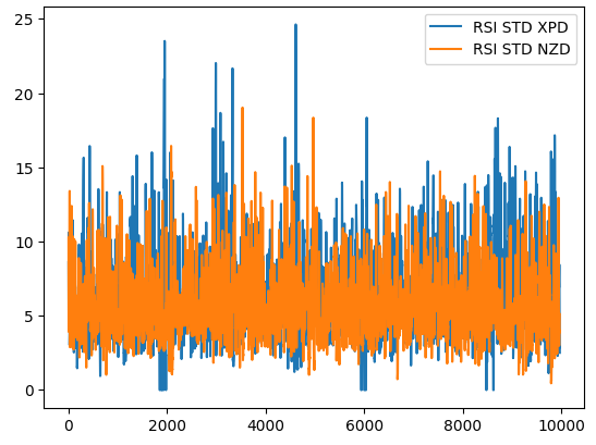
图1：XPDUSD市场的RSI指标滚动波动率（蓝色）和NZDUSD市场的RSI指标滚动波动率（橙色）

方法论概述

为了从我们拥有的数据中学习策略，我们首先使用Python的MetaTrader 5库收集了30万条M1数据。我们对数据进行了标记，然后将其划分为训练集和测试集。在训练集上，我们将RSI读数分成了10个区间，从0-10、11-20，一直到91-100。我们记录了价格在穿过每个RSI区间时未来的表现。训练数据显示，当价格穿过RSI的41-50区间时，价格水平最有上涨倾向；而当价格穿过61-70区间时，价格最有下跌倾向。

我们使用这个估计的转移矩阵构建了一个贪婪模型，该模型总是从先验分布中选择最可能的结果。我们简单的模型在测试集上达到了52%的准确率。这种方法的另一个优势是它的可解释性，我们可以很容易地理解模型是如何做出决策的。此外，现在在重要行业中使用的人工智能模型通常需要可解释性，你可以放心，这一类概率模型不会给你带来合规性问题。

再说我们对模型的准确率并不完全感兴趣。相反，我们更关注我们在训练集中识别出的10个区间的各自准确率。在我们的训练集中分布最高的两个区间，在验证集中并不可靠。在验证集上，我们在11-20区间买入，在71-80区间卖出时，获得了最高的准确率。这两个区间分别的准确率分别为51.4%和75.8%。我们选择这两个区间作为在NZDJPY货币对上开启买入和卖出仓位的最优区间。

最后，我们着手构建一个MQL5 EA，将我们在Python中分析的结果付诸实施。此外，我们在应用程序中实现了两种平仓方式。我们为用户提供了两种平仓选择：一种是在RSI指标穿过可能导致未平仓头寸减少的区间时平仓；另一种是在价格穿过移动平均线时平仓。

获取和清理数据

让我们开始吧，导入我们需要的库。

#Let's get started
import MetaTrader5       as mt5
import pandas            as pd
import numpy             as np
import seaborn           as sns
import matplotlib.pyplot as plt
import pandas_ta         as ta

检查终端是否可用。

初始化

成功

定义一些全局变量。

#Fetch market data
SYMBOL    = "NZDJPY"
TIMEFRAME = mt5.TIMEFRAME_M1

从终端中复制数据。

data = pd.DataFrame(mt5.copy_rates_from_pos(SYMBOL,TIMEFRAME,0,300000))

将时间格式从秒转换为其他单位。

data["time"]  = pd.to_datetime(data["time"],unit='s')

计算RSI。

data.ta.rsi(length=20,append=True)

定义我们我们要预测多久的未来。

#Define the look ahead
look_ahead = 20

对数据进行标记。

#Label the data
data["Target"] = np.nan

data.loc[data["close"] > data["close"].shift(-20),"Target"] = -1
data.loc[data["close"] < data["close"].shift(-20),"Target"] = 1

从数据中删除所有缺失值所在的行。

data.dropna(inplace=True)
data.reset_index(inplace=True,drop=True)

创建一个代表10组RSI值的向量。

#Create a dataframe 
rsi_matrix = pd.DataFrame(columns=["0-10","11-20","21-30","31-40","41-50","51-60","61-70","71-80","81-90","91-100"],index=[0])

这就是到目前为止我们数据的样式。

数据

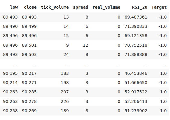
图2：我们数据结构中的一些列

将RSI矩阵的值全部初始化为0。

#Initialize the rsi matrix to 0
for i in np.arange(0,9):
    rsi_matrix.iloc[0,i] = 0

将数据分组。

#Split the data into train and test sets
train = data.loc[:(data.shape[0]//2),:]
test  = data.loc[(data.shape[0]//2):,:]

现在我们将遍历训练数据集，观察每一个RSI读数以及相应的价格水平在未来的变化。如果RSI读数为11，并且价格水平在未来上涨了20个单位，我们将在我们的RSI矩阵中将对应的11-20列增加1。此外，每当价格水平下跌时，我们将该列的值减少1。直观上，我们很快就能理解，在最终结果中，任何具有正值的列都对应于一个倾向于导致价格上涨的RSI水平，而具有负值的列则相反。

for i in np.arange(0,train.shape[0]):
    #Fill in the rsi matrix, what happened in the future when we saw RSI readings below 10?
    if((train.loc[i,"RSI_20"] <= 10)):
        rsi_matrix.iloc[0,0] = rsi_matrix.iloc[0,0] + train.loc[i,"Target"]
    #What tends to happen in the future, after seeing RSI readings between 11 and 20?
    if((train.loc[i,"RSI_20"] > 10) & (train.loc[i,"RSI_20"] <= 20)):
        rsi_matrix.iloc[0,1] = rsi_matrix.iloc[0,1] + train.loc[i,"Target"]
    #What tends to happen in the future, after seeing RSI readings between 21 and 30?
    if((train.loc[i,"RSI_20"] > 20) & (train.loc[i,"RSI_20"] <= 30)):
        rsi_matrix.iloc[0,2] = rsi_matrix.iloc[0,2] + train.loc[i,"Target"]
    #What tends to happen in the future, after seeing RSI readings between 31 and 40?
    if((train.loc[i,"RSI_20"] > 30) & (train.loc[i,"RSI_20"] <= 40)):
        rsi_matrix.iloc[0,3] = rsi_matrix.iloc[0,3] + train.loc[i,"Target"]
    #What tends to happen in the future, after seeing RSI readings between 41 and 50?
    if((train.loc[i,"RSI_20"] > 40) & (train.loc[i,"RSI_20"] <= 50)):
        rsi_matrix.iloc[0,4] = rsi_matrix.iloc[0,4] + train.loc[i,"Target"]
    #What tends to happen in the future, after seeing RSI readings between 51 and 60?
    if((train.loc[i,"RSI_20"] > 50) & (train.loc[i,"RSI_20"] <= 60)):
        rsi_matrix.iloc[0,5] = rsi_matrix.iloc[0,5] + train.loc[i,"Target"]
    #What tends to happen in the future, after seeing RSI readings between 61 and 70?
    if((train.loc[i,"RSI_20"] > 60) & (train.loc[i,"RSI_20"] <= 70)):
        rsi_matrix.iloc[0,6] = rsi_matrix.iloc[0,6] + train.loc[i,"Target"]
    #What tends to happen in the future, after seeing RSI readings between 71 and 80?
    if((train.loc[i,"RSI_20"] > 70) & (train.loc[i,"RSI_20"] <= 80)):
        rsi_matrix.iloc[0,7] = rsi_matrix.iloc[0,7] + train.loc[i,"Target"]
    #What tends to happen in the future, after seeing RSI readings between 81 and 90?
    if((train.loc[i,"RSI_20"] > 80) & (train.loc[i,"RSI_20"] <= 90)):
        rsi_matrix.iloc[0,8] = rsi_matrix.iloc[0,8] + train.loc[i,"Target"]
    #What tends to happen in the future, after seeing RSI readings between 91 and 100?
    if((train.loc[i,"RSI_20"] > 90) & (train.loc[i,"RSI_20"] <= 100)):
        rsi_matrix.iloc[0,9] = rsi_matrix.iloc[0,9] + train.loc[i,"Target"]

这是训练数据集上的计数分布。我们遇到了第一个问题：在91-100区间中没有任何训练观测值。因此，我决定假设，由于相邻区间都导致价格水平下跌，我们将给这个区间分配一个任意的负值。

rsi_matrix

0-10	11-20	21-30	31-40	41-50	51-60	61-70	71-80	81-90	91-100
4.0	47.0	221.0	1171.0	3786.0	945.0	-1159.0	-35.0	-3.0	NaN

我们可以可视化这个分布。结果显示，价格大部分时间都处于31-70区间。这对应于RSI值的中间部分。正如我们之前提到的，价格在41-50区间表现出强烈的上涨趋势，而在61-70区间表现出强烈的下跌趋势。然而，这些似乎只是训练数据的偶然现象，因为在验证数据上这种关系并不成立。

sns.barplot(rsi_matrix)

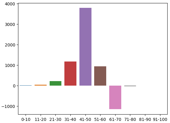
图3：RSI区间观察到的效果分布

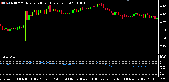
图4：迄今为止我们转换的可视化表示

现在我们将评估我们的模型在验证数据上的准确率。首先，重置训练数据的索引。

test.reset_index(inplace=True,drop=True)

为我们的模型预测创建一列。

test["Predictions"]  = np.nan

填充我们模型的预测结果。

for i in np.arange(0,test.shape[0]):
    #Fill in the predictions
    if((test.loc[i,"RSI_20"] <= 10)):
        test.loc[i,"Predictions"] = 1
    
    if((test.loc[i,"RSI_20"] > 10) & (test.loc[i,"RSI_20"] <= 20)):
        test.loc[i,"Predictions"] = 1
    
    if((test.loc[i,"RSI_20"] > 20) & (test.loc[i,"RSI_20"] <= 30)):
        test.loc[i,"Predictions"] = 1
        
    if((test.loc[i,"RSI_20"] > 30) & (test.loc[i,"RSI_20"] <= 40)):
        test.loc[i,"Predictions"] = 1

    if((test.loc[i,"RSI_20"] > 40) & (test.loc[i,"RSI_20"] <= 50)):
        test.loc[i,"Predictions"] = 1

    if((test.loc[i,"RSI_20"] > 50) & (test.loc[i,"RSI_20"] <= 60)):
        test.loc[i,"Predictions"] = 1

    if((test.loc[i,"RSI_20"] > 60) & (test.loc[i,"RSI_20"] <= 70)):
        test.loc[i,"Predictions"] = -1

    if((test.loc[i,"RSI_20"] > 70) & (test.loc[i,"RSI_20"] <= 80)):
        test.loc[i,"Predictions"] = -1

    if((test.loc[i,"RSI_20"] > 80) & (test.loc[i,"RSI_20"] <= 90)):
        test.loc[i,"Predictions"] = -1

    if((test.loc[i,"RSI_20"] > 90) & (test.loc[i,"RSI_20"] <= 100)):
        test.loc[i,"Predictions"] = -1

验证我们没有任何空值。

test.loc[:,"Predictions"].isna().any()

失败

让我们使用 pandas 来描述模型的预测与目标之间的关系。最常见的值是 True，这是一个良好的指标。

(test["Target"] == test["Predictions"]).describe()

count     148636
unique         2
top         True
freq       77409
dtype: object

让我们来评估一下模型的准确性。

#Our estimation of the model's accuracy
((test["Target"] == test["Predictions"]).describe().freq / (test["Target"] == test["Predictions"]).shape[0])

0.5207957695309346

我们关注的是这10个RSI区间的准确率。

val_err = []

在每个区间就准确率。

val_err.append(test.loc[(test["RSI_20"] < 10) & (test["Predictions"] == test["Target"])].shape[0] / test.loc[test["RSI_20"] < 10].shape[0])
val_err.append(test.loc[((test["RSI_20"] <= 20) & (test["RSI_20"] > 10)) & (test["Predictions"] == test["Target"])].shape[0] / test.loc[((test["RSI_20"] <= 20) & (test["RSI_20"] > 10))].shape[0])
val_err.append(test.loc[((test["RSI_20"] <= 30) & (test["RSI_20"] > 20)) & (test["Predictions"] == test["Target"])].shape[0] / test.loc[((test["RSI_20"] <= 30) & (test["RSI_20"] > 20))].shape[0])
val_err.append(test.loc[((test["RSI_20"] <= 40) & (test["RSI_20"] > 30)) & (test["Predictions"] == test["Target"])].shape[0] / test.loc[((test["RSI_20"] <= 40) & (test["RSI_20"] > 30))].shape[0])
val_err.append(test.loc[((test["RSI_20"] <= 50) & (test["RSI_20"] > 40)) & (test["Predictions"] == test["Target"])].shape[0] / test.loc[((test["RSI_20"] <= 50) & (test["RSI_20"] > 40))].shape[0])
val_err.append(test.loc[((test["RSI_20"] <= 60) & (test["RSI_20"] > 50)) & (test["Predictions"] == test["Target"])].shape[0] / test.loc[((test["RSI_20"] <= 60) & (test["RSI_20"] > 50))].shape[0])
val_err.append(test.loc[((test["RSI_20"] <= 70) & (test["RSI_20"] > 60)) & (test["Predictions"] == test["Target"])].shape[0] / test.loc[((test["RSI_20"] <= 70) & (test["RSI_20"] > 60))].shape[0])
val_err.append(test.loc[((test["RSI_20"] <= 80) & (test["RSI_20"] > 70)) & (test["Predictions"] == test["Target"])].shape[0] / test.loc[((test["RSI_20"] <= 80) & (test["RSI_20"] > 70))].shape[0])
val_err.append(test.loc[((test["RSI_20"] <= 90) & (test["RSI_20"] > 80)) & (test["Predictions"] == test["Target"])].shape[0] / test.loc[((test["RSI_20"] <= 90) & (test["RSI_20"] > 80))].shape[0])
val_err.append(test.loc[((test["RSI_20"] <= 100) & (test["RSI_20"] > 90)) & (test["Predictions"] == test["Target"])].shape[0] / test.loc[((test["RSI_20"] <= 100) & (test["RSI_20"] > 90))].shape[0])

绘制我们的准确率。红色线是我们50%的临界点，任何低于这条线的RSI区间可能并不可靠。我们可以清楚地观察到最后一个区间的得分为1，完美无缺。然而，回想一下，这对应于我们在超过10万分钟的训练数据中从未出现过的91-100区间。因此，这个区间可能很少见，不符合我们的交易需求。11-20区间的准确率为75%，在我们的看涨区间中是最高的。同样，71-80区间在所有看跌区间中准确率最高。

plt.plot(val_err)
plt.plot(fifty,'r')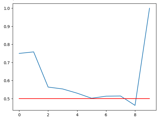

图5：可视化我们的验证准确率

我们在不同RSI区间的验证准确率。请注意，我们在91-100区间获得了100%的准确率。回想一下，我们的训练集大约有10万行数据，但我们并没有观察到该区间内的任何RSI读数。因此，我们可以得出结论，价格很少达到这些极端水平，所以这个结果可能并不是我们的最优选择。

0-10	11-20	21-30	31-40	41-50	51-60	61-70	71-80	81-90	91-100
0.75	0.75	0.56	0.55	0.53	0.50	0.51	0.51	0.46	1.0

构建我们的深度马尔可夫模型

到目前为止，我们构建的模型仅从过去的数据分布中学习。我们是否可以通过堆叠一个更灵活的学习器来增强这一策略，以学习使用我们的马尔可夫模型的最优策略呢？让我们训练一个深度神经网络，将马尔可夫模型的预测结果作为输入，而观察到的价格水平变化将作为目标值。为了有效地完成这项任务，我们需要将我们的训练集分成两部分。我们将仅使用训练集的第一部分来拟合我们的新马尔可夫模型。我们的神经网络将基于马尔可夫模型对训练集第一部分的预测以及相应的价格水平变化来进行拟合。

我们观察到，无论是我们的神经网络还是简单的马尔可夫模型，都优于直接从OHLC市场报价中学习价格水平变化的相同神经网络。这些结论是基于我们在训练过程中未使用的测试数据得出的。令人惊讶的是，我们的深度神经网络和简单的马尔可夫模型表现相当。因此，这可以被视为一种激励，促使我们付出更多努力，以超越马尔可夫模型设定的基准。

让我们开始吧，导入我们需要的库。

#Let us now try find a machine learning model to learn how to optimally use our transition matrix
from sklearn.neural_network import MLPClassifier
from sklearn.metrics import accuracy_score
from sklearn.model_selection import train_test_split,TimeSeriesSplit

现在，我们需要对我们的训练数据执行训练集和测试集的划分。

#Now let us partition our train set into 2 halves 
train , train_val = train_test_split(train,shuffle=False,test_size=0.5)

在新的训练集上拟合马尔可夫模型。

#Now let us recalculate our transition matrix, based on the first half of the training set
rsi_matrix.iloc[0,0] = train.loc[(train["RSI_20"] < 10) & (train["Target"] == 1)].shape[0] / train.loc[(train["RSI_20"] < 10)].shape[0]
rsi_matrix.iloc[0,1] = train.loc[((train["RSI_20"] > 10) & (train["RSI_20"] <=20)) & (train["Target"] == 1)].shape[0] / train.loc[((train["RSI_20"] > 10) & (train["RSI_20"] <=20))].shape[0]
rsi_matrix.iloc[0,2] = train.loc[((train["RSI_20"] > 20) & (train["RSI_20"] <=30)) & (train["Target"] == 1)].shape[0] / train.loc[((train["RSI_20"] > 20) & (train["RSI_20"] <=30))].shape[0]
rsi_matrix.iloc[0,3] = train.loc[((train["RSI_20"] > 30) & (train["RSI_20"] <=40)) & (train["Target"] == 1)].shape[0] / train.loc[((train["RSI_20"] > 30) & (train["RSI_20"] <=40))].shape[0]
rsi_matrix.iloc[0,4] = train.loc[((train["RSI_20"] > 40) & (train["RSI_20"] <=50)) & (train["Target"] == 1)].shape[0] / train.loc[((train["RSI_20"] > 40) & (train["RSI_20"] <=50))].shape[0]
rsi_matrix.iloc[0,5] = train.loc[((train["RSI_20"] > 50) & (train["RSI_20"] <=60)) & (train["Target"] == 1)].shape[0] / train.loc[((train["RSI_20"] > 50) & (train["RSI_20"] <=60))].shape[0]
rsi_matrix.iloc[0,6] = train.loc[((train["RSI_20"] > 60) & (train["RSI_20"] <=70)) & (train["Target"] == 1)].shape[0] / train.loc[((train["RSI_20"] > 60) & (train["RSI_20"] <=70))].shape[0]
rsi_matrix.iloc[0,7] = train.loc[((train["RSI_20"] > 70) & (train["RSI_20"] <=80)) & (train["Target"] == 1)].shape[0] / train.loc[((train["RSI_20"] > 70) & (train["RSI_20"] <=80))].shape[0]
rsi_matrix.iloc[0,8] = train.loc[((train["RSI_20"] > 80) & (train["RSI_20"] <=90)) & (train["Target"] == 1)].shape[0] / train.loc[((train["RSI_20"] > 80) & (train["RSI_20"] <=90))].shape[0]

rsi_matrix

0-10	11-20	21-30	31-40	41-50	51-60	61-70	71-80	81-90	91-100
1.0	0.655172	0.541701	0.536398	0.53243	0.516551	0.460306	0.491154	0.395349	0

我们可以将这个概率分布可视化。回想一下，这些数值代表价格在穿过每个RSI区间的20分钟后，价格上涨的概率。红色线代表50%的水平。所有高于50%水平的区间是看涨的，所有低于50%水平的区间是看跌的。根据训练数据的第一部分，我们可以假设这是正确的。

#From the training set, it appears that RSI readings above 61 are bearish and RSI readings below 61 are bullish
plt.plot(rsi_matrix.iloc[0,:])
plt.plot(fifty,'r')

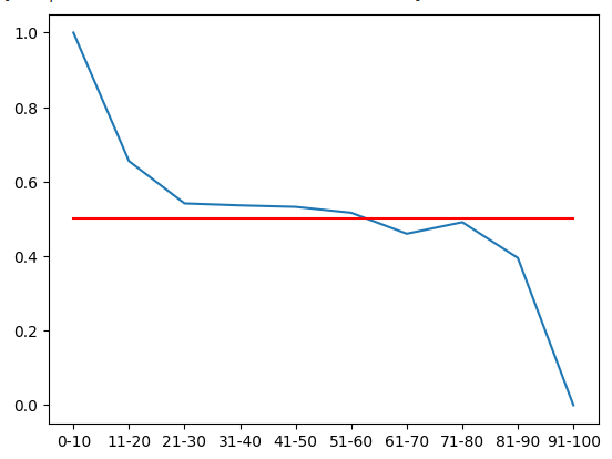
图6：从训练集的第一部分来看，所有低于61的区间是看涨的，高于61的区间是看跌的

记录马尔可夫模型做出的新预测。

#Let's now store our model's predictions
train["Predictions"] = -1
train.loc[train["RSI_20"] < 61,"Predictions"] = 1

train_val["Predictions"] = -1
train_val.loc[train_val["RSI_20"] < 61,"Predictions"] = 1

test["Predictions"] = -1
test.loc[test["RSI_20"] < 61,"Predictions"] = 1

在我们开始使用神经网络之前，通常来说，标准化和缩放数据是有帮助的。此外，我们的RSI指标范围固定在0-100之间，而我们的价格读数则没有边界。在这种情况下，标准化是必要的。

#Let's Standardize and scale our data
from sklearn.preprocessing import RobustScaler

定义我们的输入和目标。

ohlc_predictors = ["open","high","low","close","tick_volume","spread","RSI_20"]
transition_matrix = ["Predictions"]
all_predictors = ohlc_predictors + transition_matrix
target = ["Target"]

缩放数据。

scaler = RobustScaler()
scaler =  scaler.fit(train.loc[:,predictors])
train_scaled = pd.DataFrame(scaler.transform(train.loc[:,predictors]),columns=predictors)
train_val_scaled = pd.DataFrame(scaler.transform(train_val.loc[:,predictors]),columns=predictors)
test_scaled = pd.DataFrame(scaler.transform(test.loc[:,predictors]),columns=predictors)

创建数据结构以存储我们的准确率。

#Create a dataframe to store our cv error on the training set, validation training set and the test set
train_err     = pd.DataFrame(columns=["Transition Matrix","Deep Markov Model","OHLC Model","All Model"],index=np.arange(0,5)) 
train_val_err = pd.DataFrame(columns=["Transition Matrix","Deep Markov Model","OHLC Model","All Model"],index=[0]) 
test_err      = pd.DataFrame(columns=["Transition Matrix","Deep Markov Model","OHLC Model","All Model"],index=[0])

定义时间序列拆分对象。

#Create a time series split object
tscv = TimeSeriesSplit(n_splits = 5,gap=look_ahead)

对模型进行交叉验证。

model = MLPClassifier(hidden_layer_sizes=(20,10))
for i , (train_index,test_index) in enumerate(tscv.split(train_scaled)):
    #Fit the model
    model.fit(train.loc[train_index,transition_matrix],train.loc[train_index,"Target"])
    #Record its accuracy
    train_err.iloc[i,1] = accuracy_score(train.loc[test_index,"Target"],model.predict(train.loc[test_index,transition_matrix]))

#Record our accuracy levels on the validation training set
train_val_err.iloc[0,1] = accuracy_score(train_val.loc[:,"Target"],model.predict(train_val.loc[:,transition_matrix]))

#Record our accuracy levels on the test set
test_err.iloc[0,1] = accuracy_score(test.loc[:,"Target"],model.predict(test.loc[:,transition_matrix]))

#Our accuracy levels on the training set
train_err

现在让我们观察我们的模型在训练集的验证部分上的准确率。

train_val_err.iloc[0,0] = train_val.loc[train_val["Predictions"] == train_val["Target"]].shape[0] / train_val.shape[0]
train_val_err

转换矩阵	深度马尔科夫模型	OHLC 模型	所有模型
0.52309	0.52309	0.507306	0.517291

现在，最重要的是，让我们看看我们的模型在测试数据集上的准确率。从这两个表格中我们可以看到，我们的混合深度马尔可夫模型未能胜过简单的马尔可夫模型。在我看来，这让我感到意外。这可能意味着我们训练深度神经网络的过程并不理想，或者我们总是可以搜索更广泛的候选机器学习模型。我们的结果还有一个有趣的属性，那就是使用了所有数据的模型并没有表现得最好。

好消息是我们设法超过了试图直接从市场报价中预测价格的基准。看来，马尔可夫模型的简单启发式规则有助于神经网络快速学习市场的低级结构。

test_err.iloc[0,0] = test.loc[test["Predictions"] == test["Target"]].shape[0] / test.shape[0]
test_err

转换矩阵	深度马尔科夫模型	OHLC 模型	所有模型
0.519322	0.519322	0.497127	0.496724

用MQL5来实现

为了实现基于RSI的EA，我们将首先导入我们需要的库。

//+------------------------------------------------------------------+
//|                                                     Auto RSI.mq5 |
//|                                        Gamuchirai Zororo Ndawana |
//|                          https://www.mql5.com/en/gamuchiraindawa |
//+------------------------------------------------------------------+
#property copyright "Gamuchirai Zororo Ndawana"
#property link      "https://www.mql5.com/en/gamuchiraindawa"
#property version   "1.00"

//+------------------------------------------------------------------+
//| Libraries                                                        |
//+------------------------------------------------------------------+
#include <Trade\Trade.mqh>
CTrade Trade;

现在定义我们的全局变量。

//+------------------------------------------------------------------+
//| Global variables                                                 |
//+------------------------------------------------------------------+
int rsi_handler;
double rsi_buffer[];
int ma_handler;
int system_state;
double ma_buffer[];
double bid,ask;

//--- Custom enumeration
enum close_conditions
  {
   MA_Close  = 0,
   RSI_Close
  };

我们需要从用户那里获取输入。

//+------------------------------------------------------------------+
//| Inputs                                                           |
//+------------------------------------------------------------------+
input group "Technical Indicators"
input int rsi_period = 20; //RSI Period
input int ma_period = 20; //MA Period

input group "Money Management"
input double trading_volume = 0.3; //Lot size

input group "Trading Rules"
input close_conditions user_close = RSI_Close; //How should we close the positions?

每当我们的EA首次加载时，让我们加载指标并验证它们。

//+------------------------------------------------------------------+
//| Expert initialization function                                   |
//+------------------------------------------------------------------+
int OnInit()
  {
//--- Load the indicator
   rsi_handler = iRSI(_Symbol,PERIOD_M1,rsi_period,PRICE_CLOSE);
   ma_handler = iMA(_Symbol,PERIOD_M1,ma_period,0,MODE_EMA,PRICE_CLOSE);

//--- Validate our technical indicators
   if(rsi_handler == INVALID_HANDLE || ma_handler == INVALID_HANDLE)
     {
      //--- We failed to load the rsi
      Comment("Failed to load the RSI Indicator");
      return(INIT_FAILED);
     }

//---
   return(INIT_SUCCEEDED);
  }

如果我们的应用程序未在使用中，则释放指标。

//+------------------------------------------------------------------+
//| Expert deinitialization function                                 |
//+------------------------------------------------------------------+
void OnDeinit(const int reason)
  {
//--- Release our technical indicators
   IndicatorRelease(rsi_handler);
   IndicatorRelease(ma_handler);
  }

最后，如果没有未平仓的头寸，就按照我们模型的交易规则进行操作。否则，如果有未平仓的头寸，就按照用户的指示来平仓。

//+------------------------------------------------------------------+
//| Expert tick function                                             |
//+------------------------------------------------------------------+
void OnTick()
  {
//--- Update market and technical data
   update();

//--- Check if we have any open positions
   if(PositionsTotal() == 0)
     {
      check_setup();
     }

   if(PositionsTotal() > 0)
     {
      manage_setup();
     }
  }
//+------------------------------------------------------------------+

以下函数将根据用户是否希望我们使用从RSI中学到的交易规则或简单移动平均线来平仓我们的头寸。如果用户希望我们使用移动平均线，我们将在价格穿过移动平均线时平仓我们的头寸。

//+------------------------------------------------------------------+
//| Manage our open setups                                           |
//+------------------------------------------------------------------+
void manage_setup(void)
  {
   if(user_close == RSI_Close)
     {
      if((system_state == 1) && ((rsi_buffer[0] > 71) && (rsi_buffer[80] <= 80)))
        {
         PositionSelect(Symbol());
         Trade.PositionClose(PositionGetTicket(0));
         return;
        }

      if((system_state == -1) && ((rsi_buffer[0] > 11) && (rsi_buffer[80] <= 20)))
        {
         PositionSelect(Symbol());
         Trade.PositionClose(PositionGetTicket(0));
         return;
        }
     }


   else
      if(user_close == MA_Close)
        {
         if((iClose(_Symbol,PERIOD_CURRENT,0) > ma_buffer[0]) && (system_state == -1))
           {
            PositionSelect(Symbol());
            Trade.PositionClose(PositionGetTicket(0));
            return;
           }

         if((iClose(_Symbol,PERIOD_CURRENT,0) < ma_buffer[0]) && (system_state == 1))
           {
            PositionSelect(Symbol());
            Trade.PositionClose(PositionGetTicket(0));
            return;
           }
        }
  }

以下函数将检查是否有任何有效的交易设置。也就是说，价格是否已经进入了任一个盈利区间。此外，如果用户指定使用移动平均线来平仓，那么我们将等待价格处于移动平均线的正确一侧后，再决定是否开仓。

//+------------------------------------------------------------------+
//| Find if we have any setups to trade                              |
//+------------------------------------------------------------------+
void check_setup(void)
  {

   if(user_close == RSI_Close)
     {
      if((rsi_buffer[0] > 71) && (rsi_buffer[0] <= 80))
        {
         Trade.Sell(trading_volume,_Symbol,bid,0,0,"Auto RSI");
         system_state = -1;
        }

      if((rsi_buffer[0] > 11) && (rsi_buffer[0] <= 20))
        {
         Trade.Buy(trading_volume,_Symbol,ask,0,0,"Auto RSI");
         system_state = 1;
        }
     }

   if(user_close == MA_Close)
     {
      if(((rsi_buffer[0] > 71) && (rsi_buffer[0] <= 80)) && (iClose(_Symbol,PERIOD_CURRENT,0) < ma_buffer[0]))
        {
         Trade.Sell(trading_volume,_Symbol,bid,0,0,"Auto RSI");
         system_state = -1;
        }

      if(((rsi_buffer[0] > 11) && (rsi_buffer[0] <= 20)) && (iClose(_Symbol,PERIOD_CURRENT,0) > ma_buffer[0]))
        {
         Trade.Buy(trading_volume,_Symbol,ask,0,0,"Auto RSI");
         system_state = 1;
        }
     }
  }

该函数将更新我们的技术和市场数据。

//+------------------------------------------------------------------+
//| Fetch market quotes and technical data                           |
//+------------------------------------------------------------------+
void update(void)
  {
   bid = SymbolInfoDouble(_Symbol,SYMBOL_BID);
   ask = SymbolInfoDouble(_Symbol,SYMBOL_ASK);

   CopyBuffer(rsi_handler,0,0,1,rsi_buffer);
   CopyBuffer(ma_handler,0,0,1,ma_buffer);
  }
//+------------------------------------------------------------------+

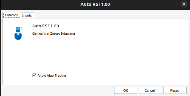
图7：我们的EA

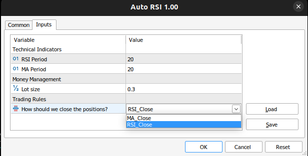
图8：我们的EA应用

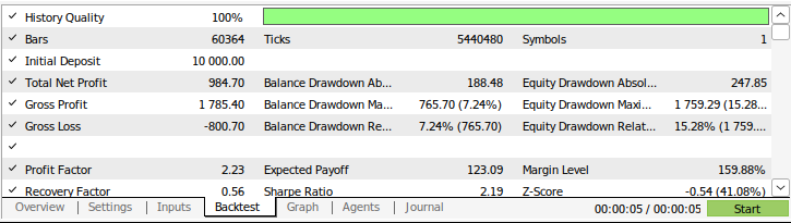
图9：策略回测结果

结论

在本文中，我们展示了简单概率模型的力量。令人惊讶的是，我们未能通过从简单马尔可夫模型的错误中学习来超越它。然而，如果你一直在密切关注这个系列文章，那么你可能会认同我的观点，即我们现在正朝着正确的方向前进。我们正在逐步积累一组比直接建模价格本身更容易建模的算法，同时这些算法在信息量上与直接对价格本身建模相当。请继续关注接下来的讨论，我们将尝试学习如何超越简单的马尔可夫模型。

本文由MetaQuotes Ltd译自英文
原文地址： https://www.mql5.com/en/articles/16030

附加的文件 |

下载ZIP

RSI_Self_Optimizer.ipynb (131.78 KB)

Auto_RSI.mq5 (6.11 KB)

注意: MetaQuotes Ltd.将保留所有关于这些材料的权利。全部或部分复制或者转载这些材料将被禁止。

该作者的其他文章

前往讨论

重构经典策略（第九部分）：多时间框架分析（第二部分）

在今天的讨论中，我们探讨了多时间框架分析的策略，以确定我们的人工智能（AI）模型在哪个时间框架上表现最优。分析结果表明，在欧元兑美元（EURUSD）货币对上，月度和小时时间框架生成的模型具有相对较低的误差率。我们利用这一优势，开发了一个交易算法，该算法在月度时间框架上进行人工智能预测，并在小时时间框架上执行交易。

大气云模型优化（ACMO）：实战

在本文中，我们将继续深入研究大气云模型优化（ACMO）算法的实现。特别是，我们将讨论两个关键方面：云向低压区域的移动以及降雨模拟，包括液滴的初始化及其在云中的分布。我们还将研究其他在管理云的状态以及确保它们与环境相互作用方面发挥重要作用的方法。

MQL5 简介（第 9 部分）：理解和使用 MQL5 中的对象

学习使用当前和历史数据在 MQL5 中创建和自定义图表对象。本基于项目的指南可帮助您可视化交易并实际应用 MQL5 概念，从而更容易构建适合您交易需求的工具。

创建 MQL5-Telegram 集成 EA 交易（第 4 部分）：模块化代码函数以增强可重用性

在本文中，我们将现有的用于从 MQL5 向 Telegram 发送消息和截图的代码重构为可重复使用的模块化函数。这将简化流程，实现跨多个实例的更高效执行和更轻松的代码管理。